XGBoost: Boosting Your Machine Learning with Extreme Gradient Boosting

Introduction 

First of all, XGBoost stands for Extreme Gradient Boosting, so as its name suggests, it’s a variant of the gradient boosting technique, which takes several weak models and adds them to a strong one to improve the predictions by learning from the mistakes made by the previous models.

XGBoost is a ML technique based on the decision tree model and the principle of boosting. What does this mean? Think of it as a bunch of models (weak decision trees) combined with each other to create a strong one (boosting method; in the previous publication, we talked about the bagging method, and we’ve mentioned this one, but boosting is combining models in such a manner that the last one gains experience from its predecessor).

So in summary, a set of weak decision models is processed one after another to enhance the prediction of the XGBoost model.

Now, let’s see the architecture of this famous model (and I said that because the XGBoost model has achieved a state-of-the-art result among other models). In the next figure, we unlock the power of this algorithm.

XGBoost architecture (the rights belong to AIblogger)

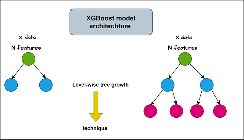
The level-wise tree growth gives XGBoost the power to get more insights about the data and predict more reliable output.

Programming 

Now let’s take us to the next level, we will be writing codes to compile the XGBoost model and unlock the secrets behind its architecture.

first of all, we need to install the XGBoost library, and to do that we should have anaconda, or any other compiler installed in your machine, go to the shell and write the next command to install XGBoost library.

pip install xgboost 
# or 
conda install xgboost
#or 
conda install -c conda-forge xgboost

Now that we have installed correctly Xgboost library, we dive into coding.

in this tutorial I will use the iris dataset as the previous lesson to compare between the results and get an idea about the power of each one.

if you want to get more information about the used dataset (Iris dataset) in random forest refer to my blog post: 

From Beginner to Pro: Mastering Random Forest with applications.
Introduction In my simple English language, if I would explain an algorithm like Random Forest, I would say that is the…easy2learnai.blogspot.com

or this medium post:

From Beginner to Pro: Mastering Random Forest with applications
Introductionmohamedtahar-fortas.medium.com

we will be doing this:

1. import the necessary libraries (and this is not crucial for the first lines of code because you will learn it alone, you will import the needed libraries when you need to use it, but there some of them are always used)
2. Load the Iris dataset using Pandas.
3. Split the dataset into features (X) and labels (y).
4. Split the data into training and testing sets using train_test_split from scikit-learn.

let’s code it:

import pandas as pd
import numpy as np
from sklearn.model_selection import train_test_split
from sklearn.metrics import accuracy_score
import xgboost as xgb
from sklearn.datasets import load_iris


# Load the Iris dataset
data = load_iris()
X = data.data
y = data.target
# Split the data into training and testing sets
X_train, X_test, y_train, y_test = train_test_split(X, y, test_size=0.2, random_state=42)

for the test size we’ve used the same as the previous time (20%<=> 0.2 for test, 80%<=>0.8 for train)

Each model has a set of parameters to tune to get the best results, in the Random Forest model we haven’t talked about this, and now also we will not talk about it ( because the hyperparameter tuning technique are so vast we can’t detail all of them here, but in case if you want to understand it i will do my best to explain it, just don’t hesitate to mention that in comments)

with this model as the previous model, we will use its default parameters to only show the results, and in future posts we will focus on that task.

the default parameters for XGBoost are the following:

params = {
    # Parameters that we are going to tune.
    'max_depth':6,
    'n_estimators': 100,
    'eta':.3,
    'subsample': 1,
    'colsample_bytree': 1,
}

let’s continue with creating the model, and we won’t specify the parameters because are already specified as default:

#The simplet XGboost model you everseen 
Xgb = xgb.XGBClassifier()

now, after we have created our model, we will fit it to the iris data, we will take as input X_train and y_train to train the model, then we will use the model in prediction as follow :

Xgb.fit(X_train, y_train)
y_pred = Xgb.predict(X_test)

Finally, we will then evaluate the model prediction power with the accuracy metric:

# Evaluate the accuracy of the classifier
accuracy = accuracy_score(y_test, y_pred)
print("Accuracy:", accuracy)

and boom this is the results :

The results of XGBoost 

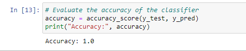
the results show that Xgboost has predicted the test data perfectly, so all the classes are correct (predicted with Xgboost) compared to the observed data (y_test).

Conclusion 

As you can see, the Xgboost is an effective model that has produced cutting-edge outcomes in a variety of applications (if you want to use it with different data sets, let me know so I can create a lesson about it).

As we previously stated, we did not modify its parameters in this lesson, and I am confident that further interesting results might be obtained with hyperparameter tweaking.

The regularization strategy included into the code of the XGboost model, which prevents the model from overfitting and speeds up the training process, as well as the aforementioned features of the XGboost model, make it suitable for usage with massive data.

---

Finally, if you made it to the footer page, I hope you find the material there to be insightful.
Please “like,” “subscribe,” and “share” this useful material with your colleagues. If there are any misconceptions, please let us know in a comment, and we’ll take care of it.

Thanks for being here, and good luck.

for more interesting things take a look at my medium account https://mohamedtahar-fortas.medium.com/

the blog URL is: Easy2learnAI 

the facebook page is : Facebook