Unlocking Titanic Survival Secrets with Machine Learning Techniques

 

Photo by NOAA on Unsplash

Introduction

Today, I’m going to unlock the secrets of the Titanic ship, where there are survivors, but we don’t know how they survived.

However, based on the dataset provided about the Titanic trip, we could find some patterns about how the passengers survived.

First of all, we should define exactly what the Titanic dataset is. The Titanic dataset, or the survival dataset of the Titanic ship, is a dataset that describes the status of the passengers based on their information, like passenger ID, whether they survived or not (1 = survived, 0 = did not survive), age, sex, name, P class (the ticket class), and so on. All of these properties make up what we call features in data science. The target in this dataset is the survived status. When using ML algorithms, our goal is to predict exactly if a passenger with specified features could survive or not based on the learned patterns.

Exploratory data analysis 

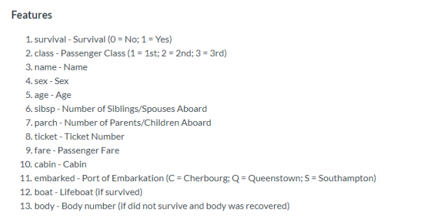
Let’s delve into a brief description of the features used in this dataset:

features of the dataset (from Titanic dataset of Kaggle competition included in the data sheet )

On this trip, there were 1502 out of 2224 survivors. And maybe you ask why the survivors survived (is there any relation between passengers and their based information?) and we hope to answer the next question, asked by the Kaggle community during the competition:

“What sorts of people were more likely to survive?”

Now, we will upload the dataset (train, test and gender submissions are downloaded from Kaggle)

import pandas as pd

train = pd.read_csv("train.csv")
test = pd.read_csv("test.csv") 
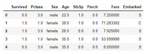
train.head()# train.shape (891, 12) 
test.head() # test.shape (418, 11)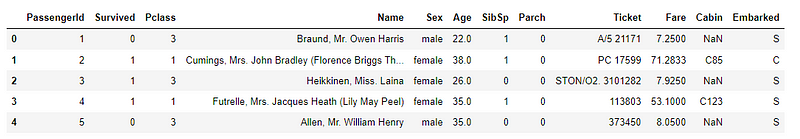

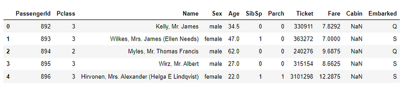
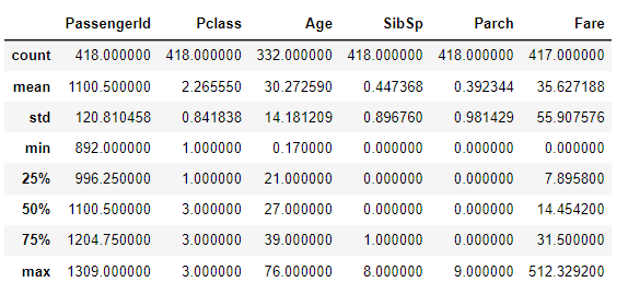
Train data 

Test data 

By using Pandas in Python, we could get a statistical description of the data we get by typing this command:

train.describe()
test.describe()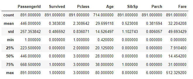

Train description 

Test description

Data preprocessing

Missing values

First of All, we should know if there are some null values or missing values to handle this problem before applying any ML model.

train.isnull().sum()
test.isnull().sum()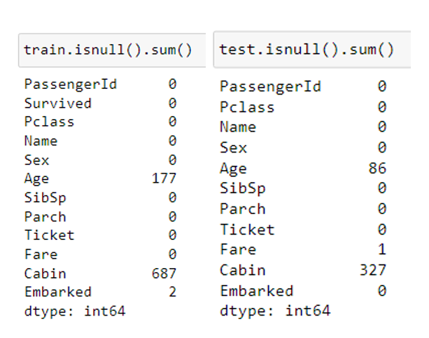

The null values in train and test datasets

As you can see, the age in the two datasets has missing values. To handle this problem, we could use data imputing techniques like zeros, mean, median, or interpolation, or we could drop the rows containing these missing values (but this is not recommended because it reduces the data size).

We have chosen to fill the missing values by 0 to save time (and this is only a choice, you could use whatever you want and compare between all of them), and this is how we do it:

train = train.fillna(0)
test = test.fillna(0)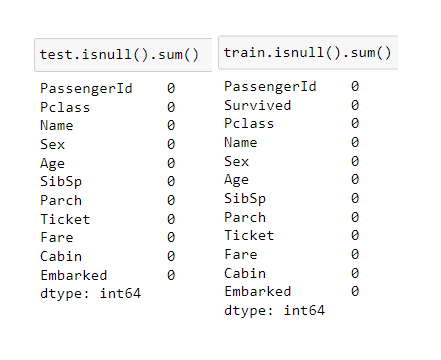

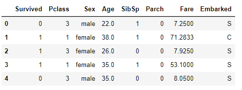
imputing Missing values 

As you know, Ticket, passenger ID, and Name have no meaning when dealing with ML models; hence, we should omit them.

and the data should look like this:

train data (the same for test)

Also, we should change the data types to float to simplify the work with the features in the model, and this is how it should look:

Train data (the same for test)

One Hot Encoding

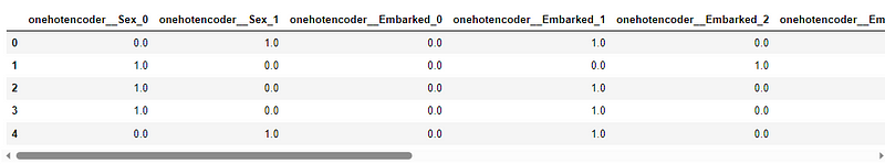
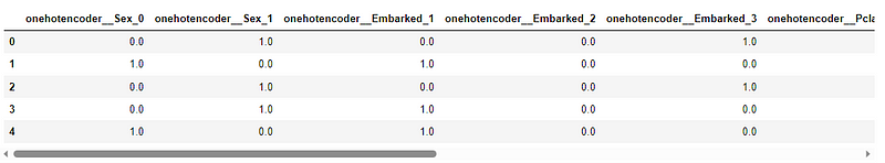
Now, if you notice, there are columns that contain categorical data; however, the ML model could not recognize categorical data. For this issue, we should transform this class data to numeric data, and for this task, we have some algorithms like One Hot Encoding and Word Embedding. In this case, we chose to use the One Hot Encoder because it’s easy (this is a method of coding class data to be used as numeric data, where the encoder assigns 0 or 1 to each class based on its presence in that row).

Train and test are the same processes (just change train to test data in the code below):

from sklearn.compose import make_column_transformer
from sklearn.preprocessing import OneHotEncoder

train['Sex'].replace('male', 1,inplace=True)
train['Sex'].replace('female', 0,inplace=True)
train['Embarked'].replace('S', 1,inplace=True)
train['Embarked'].replace('C', 2,inplace=True)
train['Embarked'].replace('Q', 3,inplace=True)

ohe = OneHotEncoder()
transformer = make_column_transformer((ohe, ['Sex', 'Embarked','Pclass']), remainder='passthrough')
transformed = transformer.fit_transform(train)

#reset the encoded data to original features data
transformed_X = pd.DataFrame(transformed, columns = transformer.get_feature_names_out())
train = transformed_X

We obtained the following results:

Encoded Train

Encoded Test

Data Normalization (MinMaxScaler)

In addition to this process of encoding, we should normalize the data to not allow the model to give chances to high values rather than low ones (by normalizing, we mean making the range of all the data values between zero and one). And it’s done as below:

from sklearn.preprocessing import MinMaxScaler

mms = MinMaxScaler()
train = mms.fit_transform(train)
train = pd.DataFrame(train, columns = transformer.get_feature_names_out())

After all of these transformations, we should go for splitting the data into training and validation (80% for training, 20 % for validation), and to do this, we call the train_test_split function:

from sklearn.model_selection import train_test_split

#0.2 means 20% for validation
train, val = train_test_split(train, test_size = 0.2 )

Drop the survived classes from the list because are the targets
train_X = train.drop(['remainder__Survived'], axis = 1)
train_Label = train['remainder__Survived']

val_X = val.drop(['remainder__Survived'], axis = 1)
val_Label = val['remainder__Survived']

Train the Model 

After completing all the data preprocessing techniques, we could apply the model that we wanted to use.

As you notice above, I didn’t talk about the chosen model for prediction, and this is because data preprocessing is a crucial step before any model choice.

In this task, I will compare two models that I’ve applied before (in the previous posts on the Iris dataset, RF and XGBoost), to know which one is more accurate than the other.

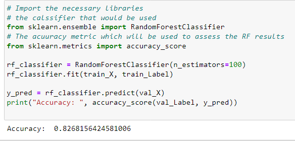
Let's delve into programming RF and XGBoost: 

This is RF results:

And this is XGBoost results:

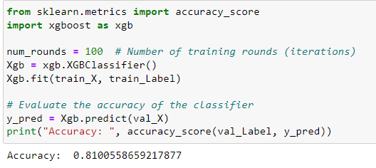
Comparing the two applied models, we should notice that the two are very good and have almost the same results, but the Random Forest is better performing than Xgboost.

In this training, I didn’t tune these models, maybe of you applied random search or grid search to tune them you would find another result, because hyperparameter tuning show the in-fact power of any model you train.

We haven’t used the test data for prediction because the ground truth data are on Kaggle, and you should place your model on that platform to get the test accuracy of the applied models.

Conclusion

In this tutorial, I’ve applied almost all the data analysis tools to the Titanic dataset, and these are almost all the techniques used. There are other techniques that I mentioned above, so if you want any details on such techniques, don’t hesitate to comment, and I’ll take care of it.

If you read this sentence, then I want to pass on my deepest thanks to you for reading this article, and if you find it helpful, please take action and share it with your friends.

#artificialIntelligence #machinelearning #datascience