From Beginner to Pro: Mastering Random Forest with applications

Introduction

In my simple English language, if I would explain an algorithm like Random Forest, I would say that is the most used algorithm in the field of AI, this machine learning architecture is based on the principle of decision trees which is a powerful idea used in classification or regression tasks, and its bases are on the decision made on each node.

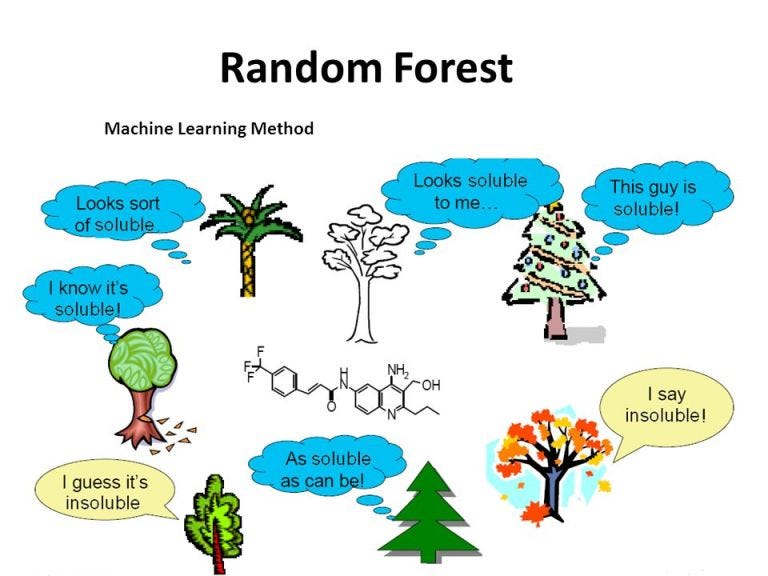
As you see in the next figure, each tree trying to guess if the chemical material is soluble or not in water !!!

from https://bigishere.wordpress.com/2018/09/22/random-forest-introduction/.

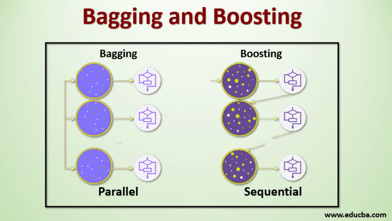
What makes RF so powerful is the combination of multiple decision trees in the same time to enhance the power of prediction of this method, as you know the RF is based on the bagging technique which explain how the trees are combined with each other to get the best output results, and this is why trees are trained in parallel (bagging) as you see in the next figure (compared to the boosting technique which we will talk about it in the next posts).

from www.educuba.com 

During the training phase, the algorithm creates a forest of decision trees. Each decision tree is trained on a bagged sample of the data, which is created by sampling with replacement. The algorithm then selects a random subset of the features for each split in the tree, which helps to split the data in a more effective way.

During the testing phase, the algorithm predicts the class or value of the target variable by aggregating the predictions of all the trees in the forest. In classification tasks, the algorithm uses a majority vote to determine the final prediction, while in regression tasks, it takes the average of the predictions.

Random Forest has several advantages:

1. It is a powerful algorithm that can handle both categorical and numerical features.
2. It performs well on a wide range of problems and is less prone to overfitting compared to individual decision trees.
3. It can handle high-dimensional data and is robust to outliers and missing values.
4. It provides estimates of feature importance, which can help in understanding the underlying patterns in the data.

so, let’s move to the programming task to ensure that RF is powerful.

Programming 

It’s obvious that the most used programming language in the field of AI is python language, and I’m sure that you know the why ?

in this post I will not talk about the python language, I will use it directly, but in case if you want to understand it here, I will do my effort to explain it in another posts don’t hesitate to request it.

In this post I will use The Iris dataset to reveal the power of RF, so if you don’t know what is the Iris dataset, read the next part carefully!!

The Iris dataset is one of the most well-known and frequently used datasets in machine learning and statistics. It was introduced by British statistician and biologist Ronald Fisher in 1936 and has since become a standard benchmark for classification tasks. The Iris dataset consists of measurements of four features (sepal length, sepal width, petal length, and petal width) from three different species of Iris flowers: Setosa, Versicolor, and Virginica. Fisher collected these measurements from 50 samples of each species, resulting in a total of 150 observations.

The goal of using the Iris dataset is typically to classify new observations into one of the three species based on their feature measurements. This makes it a popular dataset for testing and comparing different classification algorithms.

And this is the goal why we will use RF to classify the iris dataset.

Firstly, we need to preprocess the iris data set before supply it to the RF model, and this is a crucial point at any ML problem solving and should any datascientist know (data engineering).

So, first we should import some necessary libraries (Sklearn in this case ):

# Import the necessary libraries
# the calssifier that would be used 
from sklearn.ensemble import RandomForestClassifier 
#The dataset that that would be used
from sklearn.datasets import load_iris
# the train_test_split technique to split the data into train and test
from sklearn.model_selection import train_test_split
# The acuuracy metric which will be used to assess the RF results 
from sklearn.metrics import accuracy_score

after that, we will load the dataset to use it:

# Load the Iris dataset
# This is a variable named data assigned to load_iris() function 
data = load_iris()
# The data was splitted into X (input --> sepal length, 
# sepal width, petal length, and petal width) and Y (output -->
# Setosa, Versicolor, and Virginica)
X = data.data
y = data.target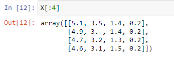

The input data X (sepal length, 

# sepal width, petal length, and petal width)

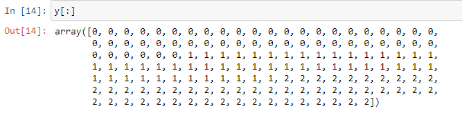The output data y (Setosa, Versicolor, and Virginica)

Assessing how well a model performs on data that hasn’t been previously observed lead us to split the data into train and test, 0.2 means 20% to test data, and 80% for the training data as well:

# Split the dataset into training and testing sets
X_train, X_test, y_train, y_test = train_test_split(X,
                                  y, test_size=0.2, random_state=42)

Now, we will create the RF model, its a simple model with n_estimators equal to 100.

n_estimators : is a hyperparameter that represents the number of decision trees to be used in the ensemble. Each decision tree in the Random Forest is trained on a random subset of the training data

# Create a Random Forest classifier with 100 trees
rf_classifier = RandomForestClassifier(n_estimators=100)

Then, as we assigned the RF classifier to a variable named rf_classifier, we will fit this model on the training subset using the following command:

# Train the classifier on the training data
rf_classifier.fit(X_train, y_train)

After that, we assess the model by this line of code on the testing data, where y_pred means the prediction values of the rf_classifier model:

# Make predictions on the testing data
y_pred = rf_classifier.predict(X_test)

And finally we get the predicion accuracy (accuracy score function) using this command:

# Evaluate the accuracy of the classifier
accuracy = accuracy_score(y_test, y_pred)
print("Accuracy:", accuracy)

The accuracy of this model was found as you see in the following figure, is 1, it means the model has predicted the classes perfectly (there is no wrong class in this prediction).

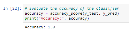The RF prediction accuracy

Conclusion

As you see, the results prove that RF is a very powerful model, this is why it is used in different applications like Natural Language Processing, Recommendation Systems, Bioinformatics, Anomaly Detection, Feature Selection …etc. Random forest show a high performance compared to another algorithms.

Finally, I hope you find this micro-tutorial very helpful, and if you want more posts like this one just comment and I will do my effort to add more useful lessons about AI and ML.

comment and share with your friends if you like the lesson, and if you want more refer to my posts on meduim Easy2learn