

Introduction
First of all, when talking about data manipulation techniques, the most famous one is pandas. So, what is Pandas? What are its capabilities? And how could we use it? Also, what are the functions inside this library? all of these questions and others will be answered in the next few paragraphs, so let’s delve right in.
Table of Contents
- What is Pandas?
- Installing Pandas
- Importing the Pandas Library
- Pandas Data Structures
4.1 Series
4.2 DataFrame
5. Data Input and Output
5.1 Reading Data
5.2 Writing Data
6. Data Manipulation with Pandas
6.1 Selecting Data
6.2 Filtering Data
6.3 Handling Missing Data
6.4 Applying Functions to Data
6.5 Grouping and Aggregating Data
6.6 Merging and Joining Data
6.7 Reshaping and Pivoting Data
6.8 Sorting Data
7. Advanced Pandas Techniques
7.1 Working with Dates and Times
7.2 Handling Categorical Data
7.3 Applying Vectorized Operations
7.4 Performance Optimization
1. What is Pandas?
Pandas is an open-source library built on top of NumPy that provides data manipulation techniques to easily read different data structures and manipulate them quickly and efficiently.
There are two types of data structures handled by this library: series, which are one dimensional data structures with labels, and DataFrames, which are two-dimensional tables with data labels.
2. Installing Pandas
The most famous method is to install it with pip. First, open the command prompt of the IDLE you use and type the following line:
pip install pandas and you finally get it installed on your machine, so go ahead and use it.
3. Importing the Pandas library
To import the library, type the first line or the second one, but typically the second is the most used one because of its ease.
import pandas # or /

import pandas as pd # to reduce the name of the library
4. Pandas Data Structures
4.1 Series
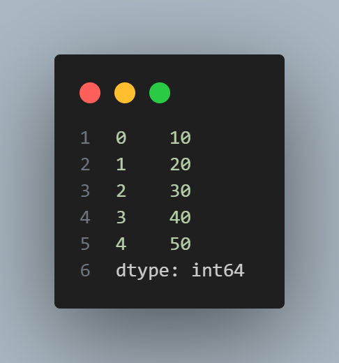
Series are a data structure like arrays, however, there are labels with these data values, and this is a brief example of it:
import pandas as pd

data = [10, 20, 30, 40, 50]
series = pd.Series(data)
print(series)
and this is the output:
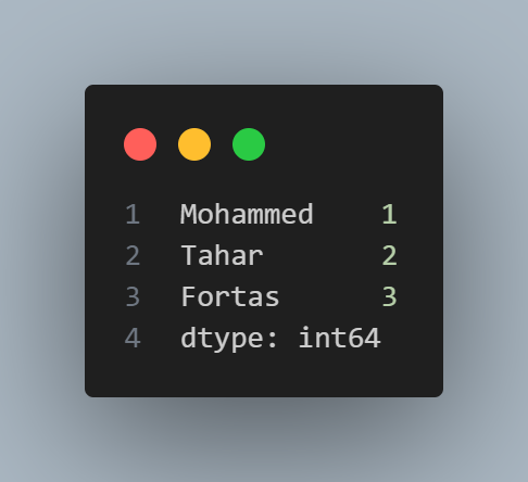
We could also, define a dictionary and then convert it to a data series as follows:
d = {'Mohammed': 1, 'Tahar': 2, 'Fortas': 3}
ser = pd.Series(data=d)
ser
and the output looks like this:
In addition, we could also construct series from arrays and lists.
4.2 DataFrame
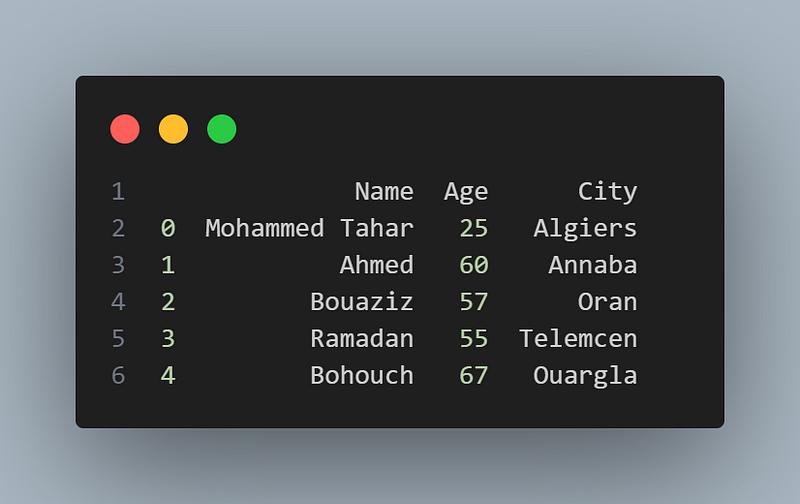
The DataFrame is the most widely used data structure in Pandas. It represents a tabular, two-dimensional data structure with labeled axes (rows and columns). Here’s an example of creating a DataFrame from a dictionary:
import pandas as pd

data = {
    'Name': ['Mohammed Tahar', 'Ahmed', 'Bouaziz', 'Ramadan', 'Bohouch'],
    'Age': [25, 60, 57, 55, 67],
    'City': ['Algiers', 'Annaba', 'Oran', 'Telemcen', 'Ouargla']
}

df = pd.DataFrame(data)
print(df)
the output:
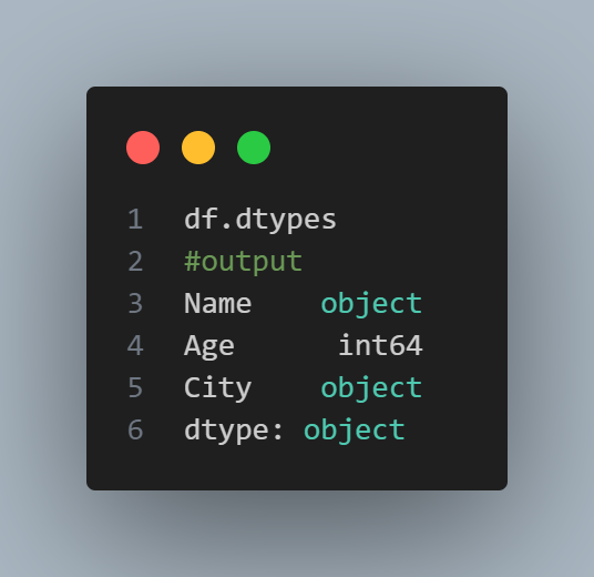
The data types of the values included in this dataframe are:
Dataframes could also be created from a NumPy array, as follows:
import numpy as np
import pandas as pd
arr = np.array([[10, 20, 30], [32, 54, 78], [89, 836, 523]])
df = pd.DataFrame(arr)
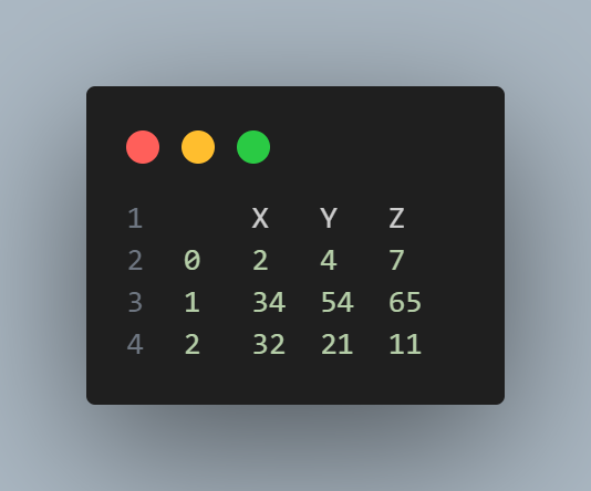
dfConstructing a dataframe from a data class
from dataclasses import make_dataclass

#create triangles and strore their coordinates in dataframe
Tri = make_dataclass('Triangle', [("X", int), ('Y', int), ('Z', int)])
pd.DataFrame([Tri(2, 4, 7), Tri(34, 54, 65), Tri(32, 21, 11])
Output:
We could also create a dataframe from Nd (n-dimensional) arrays or lists.
5. Data input and output
5.1 Reading data
Pandas offers a number of ways to read data from various file formats, including CSV, Excel, SQL databases, and more. An illustration of reading a CSV file into a DataFrame is shown below:
import pandas as pd

# data.csv is the file you want to read, and it should be in the
# same directory of this script
df = pd.read_csv('data.csv')
print(df)
The output depends on the data, and the data would be stored in the df variable. We could also read from Excel, an SQL database, or text files.
5.2 Writing data
Similarly, Pandas allows you to write data from a DataFrame to various file formats. Here’s an example of writing a DataFrame to a CSV file:
import numpy as np
import pandas as pd

arr = np.array([[10, 20, 30], [32, 54, 78], [89,  836, 523]])

df = pd.DataFrame(arr)

df.to_csv('output.csv', index=False)
The output: created file in the same directory as the script, this will write the contents of the DataFrame df to a file named "output.csv" without including the index column.
6. Data Manipulation with Pandas
6.1 Selecting data
You can select specific columns or rows of a DataFrame using indexing and slicing. Here are a few examples:
import pandas as pd
data = {
'Name': ['Mohammed Tahar', 'Ahmed', 'Bouaziz', 'Ramadan', 'Bohouch'],
'Age': [25, 60, 57, 55, 67],
'City': ['Algiers', 'Annaba', 'Oran', 'Telemcen', 'Ouargla']
}
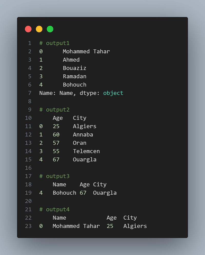
data = pd.DataFrame(data)
# Selecting a single column
column = data['Name']
column
# Selecting multiple columns
columns = data[['Age', 'City']]
columns
# Selecting columns based on conditions
filtered_rows1 = data[data['Age'] > 60]
filtered_rows1
# Selecting columns based on multiple conditions
filtered_rows2 = data[(data['Age'] > 10) & (data['City'] == 'Algiers')]
filtered_rows2the outputs: (Note that, this way, only the last line would show as a result; however, I compiled the lines one by one.)
6.2 Filtering Data
You can filter data based on specific conditions using the query() method or Boolean indexing. Here's an example:
import pandas as pd
data = {
'Name': ['Mohammed Tahar', 'Ahmed', 'Bouaziz', 'Ramadan', 'Bohouch'],
'Age': [25, 60, 57, 55, 67],
'City': ['Algiers', 'Annaba', 'Oran', 'Telemcen', 'Ouargla']
}
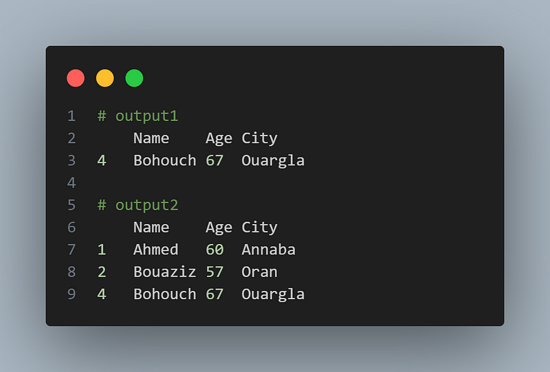
data = pd.DataFrame(data)
# Using query() method
filtered_data = data.query('Age > 60')
filtered_data
# Using Boolean indexing
filtered_data = data[data['Age'] > 55]
filtered_dataScript outputs:
6.3 Handling Missing Data
Pandas provides methods to handle missing or null values in your data. Some common techniques include:
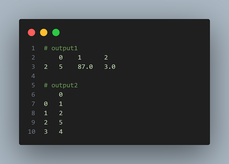
Checking for missing values:
import pandas as pd

df = pd.DataFrame([[1, None, None], [None, 3, 5], [5, 87, 3], [None, None, 3]])
# Checking for missing values
missing_values = df.isnull().sum()
# print df
df
# print the number of missing values
missing_values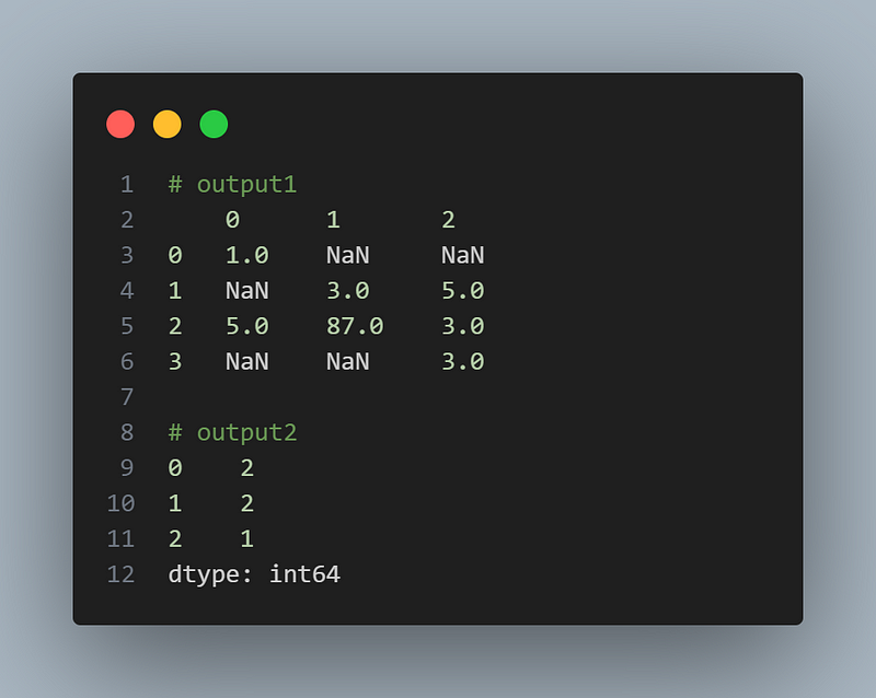
Dropping missing values:
import pandas as pd

df = pd.DataFrame([[1, None, None], [2, None, 5], [5, 87, 3], [4, None, 3]])

# Dropping rows with missing values
df.dropna()

# Dropping columns with missing values
df.dropna(axis=1)
The output:
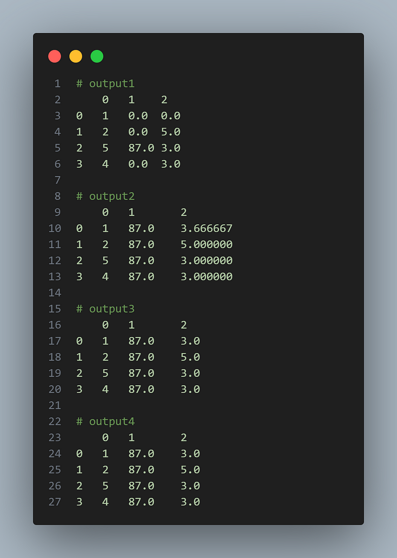
Filling missing values:
We could fill in missing values by different methods: zeros, mean, median, mode, and so on.
import pandas as pd

# Filling missing values with a specific value
value = 0  # or any other value
df.fillna(value)

# Filling missing values with mean, median, or mode
df.fillna(df.mean())
df.fillna(df.median())
df.fillna(df.mode().iloc[0])
Output:
6.4 Applying Functions to Data
You can apply functions to DataFrame columns or rows using the apply() method. Here's an example:
import pandas as pd
df = pd.DataFrame([[1, None, None], [2, None, 5], [5, 87, 3], [4, None, 3]])
df = df.fillna(df.mode().iloc[0])

# Applying a function to a column
df['X'] = df[0].apply(lambda x: x * 2 + 1 )

# Applying a function to each row
df['Y'] = df.apply(lambda row: row[1] +  row[2], axis=1)
df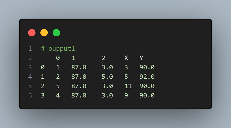
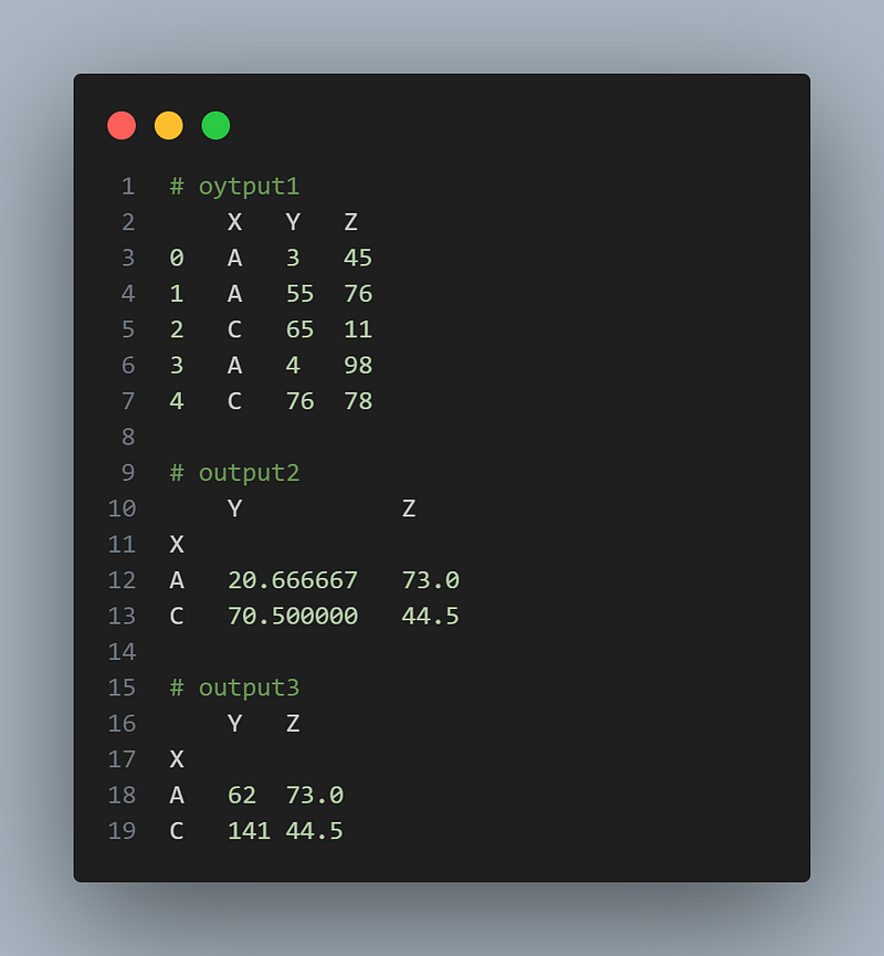
6.5 Grouping and Aggregating Data
Pandas allows you to group data based on one or more columns and perform aggregations on the grouped data. Here’s an example:
import pandas as pd
d = {'X': ['A', 'A', 'C', 'A', 'C'], 'Y': [3, 55,65, 4, 76], 'Z': [45, 76, 11, 98, 78]}
df = pd.DataFrame(d)
# Grouping data and calculating the mean
grouped_data = df.groupby(['X']).mean()
#show df
df
#show the groupby output
grouped_data

# Applying multiple aggregations on grouped data
grouped_data = df.groupby('X').agg({'Y': 'sum', 'Z': 'mean'})
grouped_data
Output:
6.6 Merging and Joining Data
You can combine multiple DataFrames based on common columns using merge or join operations. Here’s an example:
import pandas as pd

df1 = pd.DataFrame({'c':[45, 6], 'a':[2, 4], 'b': [5, 4]})
df2 = pd.DataFrame({'f':[23, 4], 'd':[34, 5], 'c':[45, 6]})
# Merging two DataFrames
merged_data =df1.merge(df2,  on='c')
# Joining two DataFrames
joined_data = df1.join(df2.set_index('c'), on='c')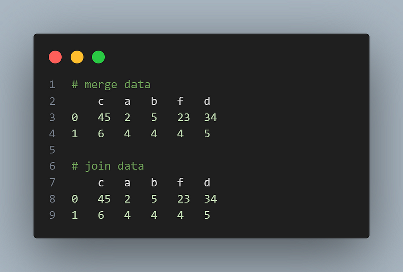
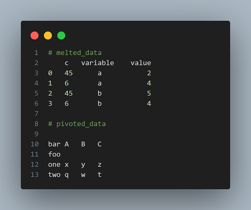
6.7 Reshaping and Pivoting Data
Pandas provides functions for reshaping and pivoting your data. Here’s an example:
import pandas as pd

df = merged_data
# Reshaping data using melt
melted_data = pd.melt(df, id_vars=['c'], value_vars=['a', 'b'])
melted_data

# Pivoting data using pivot
df = pd.DataFrame({'foo': ['one', 'one', 'one', 'two', 'two','two'],
                   'bar': ['A', 'B', 'C', 'A', 'B', 'C'],
                   'baz': [1, 2, 3, 4, 5, 6],
                   'zoo': ['x', 'y', 'z', 'q', 'w', 't']})
pivoted_data = df.pivot(index='foo', columns='bar', values='zoo')
pivoted_data
Output:
6.8 Sorting Data
You can sort your data based on one or more columns using the sort_values() method. Here’s an example:import pandas as pd
df = pd.DataFrame({'foo': ['one', 'one', 'one', 'two', 'two','two'],
'bar': ['A', 'B', 'C', 'A', 'B', 'C'],
'baz': [1, 2, 3, 4, 5, 6],
'zoo': ['x', 'y', 'z', 'q', 'w', 't']})
# Sorting data based on a single column
sorted_data = df.sort_values('baz', ascending=False)
sorted_data
# Sorting data based on multiple columns
sorted_data = df.sort_values(['bar', 'baz'], ascending=[True, False])
sorted_data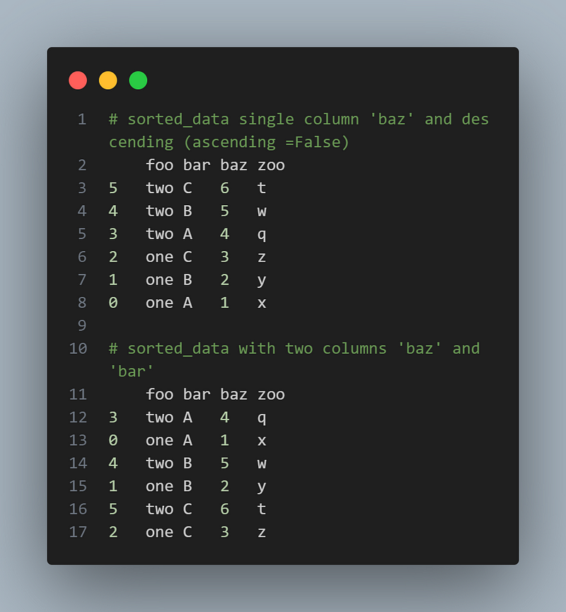
7. Advanced Pandas Techniques
In addition to the core functionalities, Pandas offers advanced techniques to handle specific scenarios. Let’s explore a few:
7.1 Working with Dates and Times
Pandas provides powerful tools for working with dates and times. You can convert strings to datetime objects, extract components, perform arithmetic operations, and more. Here’s an example:
import pandas as pd

df = pd.DataFrame({'year': [2015, 2016],
                   'month': [2, 3],
                   'day': [4, 5]})

# Converting a string column to datetime
pd.to_datetime(df)
7.2 Handling Categorical Data
Pandas supports categorical data, which can be beneficial for memory and performance optimization. You can convert columns to categorical types and perform operations specific to categorical data. Here’s an example:
import pandas as pd

df = pd.DataFrame({'f':[23, 4], 'd':[34, 5], 'c':[45, 6]})
# Converting a column to categorical type
df['f'] = df['f'].astype('category')
df.dtypes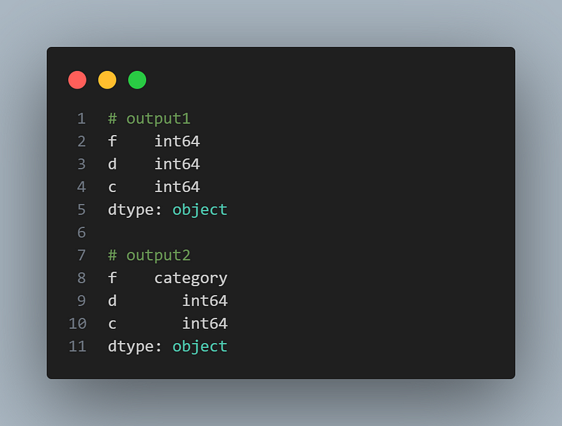
7.3 Applying Vectorized Operations
Pandas leverages NumPy’s vectorized operations, allowing you to perform computations efficiently on large datasets. Instead of looping through rows, you can apply operations to entire columns or series. Here’s an example:
import pandas as pd

df = pd.DataFrame({'f':[23, 4], 'd':[34, 5], 'c':[45, 6]})
# Applying vectorized operations
df['New_Column'] = df['f'] + df['f']
df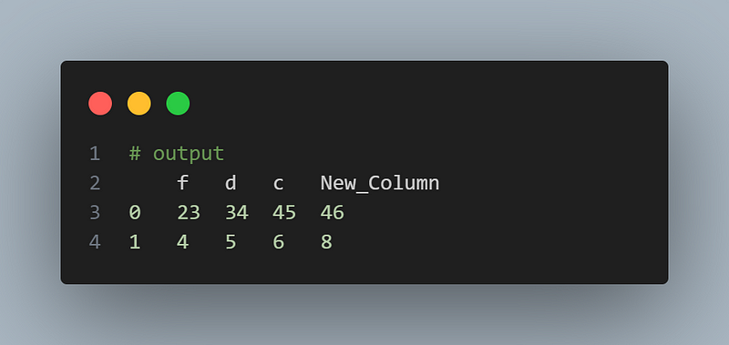
7.6 Performance Optimization
Pandas provides various techniques to optimize the performance of your data manipulation operations. Some common techniques include using vectorized operations, avoiding loops, utilizing Pandas’ built-in functions, and using appropriate data structures. Here’s an example:
import pandas as pd

df = pd.DataFrame({'a':['Mohammed', 'Tahar'], 'b':['Tahar', 'Fortas']})
X = df['a'].apply(lambda x: pd.Series(x.split('a')))
X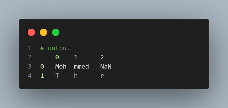
Conclusion
This blog article examined the Pandas package, an effective Python tool for handling and analyzing data. We went through the fundamentals of Pandas, such as its data structures, input/output functions, and several data manipulation strategies. In addition, we explored advanced Pandas strategies and provided some practical tips to improve your data manipulation productivity. You have a strong toolkit at your fingertips with Pandas for managing data in your projects effectively and efficiently. So go ahead and use Pandas to their full potential to further your data research!
this is my medium account: Medium account


0 Comments
Just comment!!!